Storytelling with Data - Web Analysis

Why Storytelling?
Visual analysis means exploring data visually. A story unfolds as you navigate from one visual summary into another.
You and your team have sorted through and analyzed a dense data set, made industry-relevant discoveries and created data visualizations that allow you to share those insights with others—whether other team members, current or potential clients, or the community at large. Before you present your work, think about your audience and the goals you want to achieve.
Keep in mind that the people you want to communicate with may not have the same background or technical knowledge that you do. Although eager to understand, audience members may need additional explanation, simplified insights or a more slowly paced presentation to grasp your point of view. Making the data accessible to your audience is your responsibility.
A tried-and-true method of connecting with your audience is to embed your data insights within a story. The story framework will capture your audience's attention and help you meet the business objectives driving your work.

Story Framework
Before you embark on your data journey, identify the questions you want to answer. You may have a specific question in mind or a general area you'd like to explore. As you dig into your data, you may find an entirely new or unexpected story, but it helps to have a starting point.

An example of one story framework for a web analysis example on how to visualize online campaign performance.

and the output...

Read more

Statistical p-values

When results of studies or research are reported, important decisions are made on the basis of these results. For example, new varieties are often tested against standard varieties to determine if the new varieties is more effective. Several methods of manufacturing may be compared to select the best technique to manufacture the best product. Several evidence may be examined to determine if there is a possible link between one activity and a result. In such kind of studies, results are summarized by a statistical test, and a decision about the significance of the result is based on a p-value. Therefore, it is important for the reader to know what the p-value is all about.
To describe how the p-value works, we'll use a common statistical test as an example, the Student's t-test for independent groups. For this test, subjects are randomly assigned to one of two groups. Some treatment is performed on the subjects in one group, and the other group acts as a control where no treatment or a standard treatment is given. For this example, suppose group one is given a new drug and group 2 is given then standard drug. Time to relief is measured for both groups. The outcome measurement is assumed to be a continuous variable which is normally distributed, and it is assumed that the population variance for the measure is the same for both groups.
For this example the sample mean for group one is 10 and the sample mean for group two is 12. The sample standard deviation for group one is 1.8 and the sample standard deviation for group two is 1.9. The sample size for both groups is 12. Entering this data into a statistical program will produce a t-statistic and a p-value. Calculated t = -2.65 with 22 degrees of freedom, and a p-value of 0.0147. This means that you have evidence that the mean time to relief for group one was significantly different than for group two.
To interpret this p-value, you must first know how the test was structured. In the case of this two-sided t-test, the hypotheses are:
Ho: u1 = u2 (Null hypothesis: means of two groups are equal)
Ha: u1 <> u2 (Alternative: means of the two groups are not equal)
A low p-value for the statistical test points to rejection of the null hypothesis because it indicates how unlikely it is that a test statistic as extreme as or more extreme than the one given by this data will be observed from this population if the null hypothesis is true. Since p=0.015, this means that if the population means were equal as hypothesized (under the null), there is a 15 in 1000 chance that a more extreme test statistic would be obtained using data from this population. If you agree that there is enough evidence to reject the null hypothesis, you conclude that there is significant evidence to support the alternative hypothesis.
The researcher decides what significance level to use i.e., what cutoff point will decide significance. The most commonly used level of significance is 0.05. When the significance level is set at 0.05, any test resulting in a p-value under 0.05 would be significant. Therefore, you would reject the null hypothesis in favor of the alternative hypothesis. Since you are comparing only two groups, you can look at the sample means to see which is largest. The sample mean of group one is smallest, so you conclude that medicine one acted significantly faster, on average, than medicine two. This would be reported in an article using a phrase like this: "The mean time to relief for group one was significantly smaller than for group two. (two sided t-test, t(22) = -2.65, p=0.015)."
P-values do not simple provide you with a Yes or No answer, they provide a sense of the strength of the evidence against the null hypothesis. Lower the p-value, the stronger the evidence.

Read more

Cautions about Regression and Correlation

Correlation and regression are powerful tools for describing the relationship between two variables. When you use these tools, you must be aware of their limitations.

■ Correlation and regression lines describe only linear relationships. You can do the calculations for any relationship between two quantitative variables, but the results are useful only if the scatterplot shows a linear pattern.
■ Correlation and least-squares regression lines are not resistant. Always plot your data and look for observations that may be influential.
■Extrapolation. Suppose that you have data on a child’s growth between 3 and 8 years of age. You find a strong linear relationship between age x and height y. If you fit a regression line to these data and use it to predict height at age 25 years, you will predict that the child will be 8 feet tall. Growth slows down and
then stops at maturity, so extending the straight line to adult ages is foolish. Few relationships are linear for all values of x. Don’t make predictions far outside the range of x that actually appears in your data.
■Lurking variable. the relationship between two variables can often be understood only by taking other variables into account. Lurking variables can make a correlation or regression misleading.

You should always think about possible lurking variables before you draw conclusions based on correlation or regression.

E X T R A P O L AT I O N
Extrapolation is the use of a regression line for prediction far outside the range of values of the explanatory variable x that you used to obtain the line. Such predictions are often not accurate.

L U R K I N G V A R I A B L E
A lurking variable is a variable that is not among the explanatory or response variables in a study and yet may influence the interpretation of relationships among those variables.

Read more

Statistical Terminology - Explained

We often make use of statistical techniques in the analysis of findings. Some are highly sophisticated and complex, but those most often used are easy to understand. The most common are measures of central tendency (ways of calculating averages) and correlation coefficients (measures of the degree to which one variable relates consistently to another). There are three methods of calculating averages, each of which has certain advantages and shortcomings. Take as an example the amount of personal wealth (including all assets such as houses, cars, bank accounts and investments) owned by 13 individuals. Suppose they own the following amounts:

1. £000 (zero)
2 £5,000
3. £10,000
4. £20,000
5. £40,000
6. £40 ,000
7. £40,000
8. £80,000
9. £100,000
10. £150,000
11. £200,000
12. £400,000
13. £10,000,000

The mean corresponds to the average, arrived at by adding together the personal wealth of all 13 people and dividing the result by 13. The total is £11,085,000; dividing this by 13, we reach a mean of £852,692.31. This mean is often a useful calculation because it is based on the whole range of data provided. However, it can be misleading where one or a small number of cases are very different from the majority. In the above example, the mean is not in fact an appropriate measure of central tendency, because the presence of one very large figure, £ 1 0,000,000 skews the picture. One might get the impression when using the mean to sumnarize this data that most of the people own far more than they actually do. In such instances, one of two other measures may be used. The mode is the figure that occurs most frequently in a given set of data. In our example, it is £40,000. The problem with the mode is that it does not take into account the overall distribution of the data - i.e., the range of figures covered. The most frequently occurring case in a set of figures is not necessarily representative of their distribution as a whole and thus may not be a useful average. In this case, £40,000 is too close to the lower end of the figures. The third measure is the median, which is the middle of any set of figures; here, this would be the seventh figure, again £40,000. Our example gives an odd number of figures 13. If there had been an even number - for instance, 12 - the median would be calculated by taking the mean of the two middle cases. Like the mode, the median gives no idea of the actual range of the data measured.

Sometimes a researcher will use more than one measure of central tendency to avoid giving a deceptive picture of the average. More often, he will calculate the standard deviation for the data in question. This is a way of calculating the degree of dispersal, or the range, of a set of figures - which in this case goes from zero to £10,000,000. Correlation coefficients offer a useful way of expressing how closely connected two (or more) variables are. Where two variables correlate completely, we can speak of a perfect positive correlation, expressed as 1. Where no relation is found between two variables - they have no consistent connection at all, the coefficient is zero. A perfect negative correlation, expressed as -1, exists when two variables are in a completely inverse relation to one another. Correlations of the order of 0.6 or more, whether positive or negative, are usually regarded as indicating a strong degree of connection between whatever variables are being analysed. Positive correlations on this level might be found between, say, social class background and voting behaviour.

Read more

Multicollinearity

The use and interpretation of a multiple regression model depends implicitly on the assumption that the explanatory variables are not strongly interrelated. In most regression applications the explanatory variables are not orthogonal. Usually the lack of orthogonality is not serious enough to affect the analysis. However, in some situations the explanatory variables are so strongly interrelated that the regression results are ambiguous. Typically, it is impossible to estimate the unique effects of individual variables in the regression equation. The estimated values of the coefficients are very sensitive to slight changes in the data and to the addition or deletion of variables in the equation. The regression coefficients have large sampling errors which affect both inference and forecasting that is based on the regression model. The condition of severe non-orthogonality is also referred to as the problem of multicollinearity.

The presence of multicollinearity has a number of potentially serious effects on the least squares estimates of regression coefficients. Multicollinearity also tends to produce least squares estimates that are too large in absolute value.

Remedial Measures

i) Collection of additional data: Collecting additional data has been suggested as one of the methods of combating multicollinearity. The additional data should be collected in a manner designed to break up the multicollinearity in the existing data.

ii) Model respecification: Multicollinearity is often caused by the choice of model, such as when two highly correlated regressors are used in the regression equation. In these situations some respecification of the regression equation may lessen the impact of multicollinearity. One approach to respecification is to redefine the regressors. For example, if x1, x2 and x3 are nearly linearly dependent it may be possible to find some function such as x = (x1+x2)/x3 or x = x1x2x3 that preserves the information content in the original regressors but reduces the multicollinearity.

iii) Ridge Regression: When method of least squares is used, parameter estimates are unbiased. A number of procedures have been developed for obtaining biased estimators of regression coefficients to tackle the problem of multicollinearity. One of these procedures is ridge regression. The ridge estimators are found by solving a slightly modified version of the normal equations. Each of the diagonal elements of X'X matrix are added a small quantity.

Read more

Diagnostics and Remedial Measures

The interpretation of data based on analysis of variance (ANOVA) is valid only when the following assumptions are satisfied:
1. Additive Effects: Treatment effects and block (environmental) effects are additive.
2. Independence of errors: Experimental errors are independent.
3. Homogeneity of Variances: Errors have common variance.
4. Normal Distribution: Errors follow a normal distribution.
Also the statistical tests t, F, z, etc. are valid under the assumption of independence of errors and normality of errors. The departures from these assumptions make the interpretation based on these statistical techniques invalid. Therefore, it is necessary to detect the deviations and apply the appropriate remedial measures.

• The assumption of independence of errors, i.e., error of an observation is not related to or depends upon that of another. This assumption is usually assured with the use of proper randomization procedure. However, if there is any systematic pattern in the arrangement of treatments from one replication to another, errors may be non-independent. This may be handled by using nearest neighbour methods in the analysis of experimental data.

• The assumption of additive effects can be defined and detected in the following manner:

Additive Effects: The effects of two factors, say, treatment and replication, are said to be additive if the effect of one-factor remains constant over all the levels of other factors. A hypothetical set of data from a randomized complete block (RCB) design, with 2 treatments and 2 replications, with additive effects is as

Treatment                        Replication       Replication Effect
                                         I           II            I - II
A                                    190       125            65
B                                    170       105            65
Treatment Effect (A-B)    20         20
Here, the treatment effect is equal to 20 for both replications and replication effect is 65 for both treatments.
When the effect of one factor is not constant at all the levels of other factor, the effects are said to be non-additive.

Normality of Errors: The assumptions of homogeneity of variances and normality are generally violated together. To test the validity of normality of errors for the character under study, one can take help of Normal Probability Plot, Anderson-Darling Test, D'Augstino's Test, Shapiro - Wilk's Test, Ryan-Joiner test, Kolmogrov-Smirnov test, etc. In general moderate departures from normality are of little concern in the fixed effects ANOVA as F - test is slightly affected but in case of random effects, it is more severely impacted by non-normality. The significant deviations of errors from normality, makes the inferences invalid. So before analyzing the data, it is necessary to convert the data to a scale that it follows a normal distribution. In the data from designed field experiments, we do not directly use the original data for testing of normality or homogeneity of observations because this is embedded with the treatment effects and some of other effects like block, row, column, etc. So there is need to eliminate these effects from the data before testing the assumptions of normality and homogeneity of variances. For eliminating the treatment effects and other effects we fit the model corresponding to the design adopted and estimate the residuals. These residuals are then used for testing the normality of the observations. In other words, we want to test the null hypothesis H0: errors are normally distributed against alternative hypothesis H1: errors are not normally distributed. In SAS and SPSS commonly used tests are Shapiro-Wilk test and Kolmogrov-Smirnov test. MINITAB uses three tests viz. Anderson-Darling, Ryan-Joiner, Kolmogrov-Smirnov for testing the normality of data.

Homogeneity of Error Variances: A crude method for detecting the heterogeneity of variances is based on scatter plots of means and variance or range of observations or errors, residual vs fitted values, etc.

Based on these scatter plots, the heterogeneity of variances can be classified into two types:
1. Where the variance is functionally related to mean.
2. Where there is no functional relationship between the variance and the mean.
The scatter-diagram of means and variances of observations for each treatment across the replications gives only a preliminary idea about homogeneity of error variances. Statistically the homogeneity of error variances is tested using Bartlett's test for normally distributed errors and Levene test for non-normal errors.

Remedial Measures: Data transformation is the most appropriate remedial measure, in the situation where the variances are heterogeneous and are some functions of means. With this technique, the original data are converted to a new scale resulting into a new data set that is expected to satisfy the homogeneity of variances. Because a common transformation scale is applied to all observations, the comparative values between treatments are not altered and comparison between them remains valid.

Error partitioning is the remedial measure of heterogeneity that usually occurs in experiments, where, due to the nature of treatments tested some treatments have errors that are substantially higher (lower) than others.

Here, we shall concentrate on those situations where character under study is non-normal and variances are heterogeneous. Depending upon the functional relationship between variances and means, suitable transformation is adopted. The transformed variate should satisfy the following:

1. The variances of the transformed variate should be unaffected by changes in the means. This is also called the variance stabilizing transformation.
2. It should be normally distributed.
3. It should be one for which effects are linear and additive.
4. The transformed scale should be such for which an arithmetic average from the sample is an efficient estimate of true mean.

The following are the three transformations, which are being used most commonly.

a) Logarithmic Transformation
b) Square Root Transformation
c) Arc Sine or Angular Transformation

Read more

Web Analytics - An Overview

Web analytics is the practice of measuring, collecting, analysing and reporting online data for the purposes of understanding how a web site is used by its visitors and how to optimise its usage. The focus of web analytics is to understand a site’s users, their behaviour and activities.

The study of online user behaviour and activities generates valuable marketing intelligence and provides:

• performance measures of the website against targets

• insights on user behaviours and needs, and how the site is meeting those needs

• optimisation ability to make modifications to improve the website based on the results

An average web analytics tool offers hundreds of metrics. All are interesting but only a few would be useful for measuring the website’s performance. Focus on what is important to get meaningful insights about your website, start your web analytics initiative by defining realistic and measurable objectives for your site.

A business will not be successful if the customers are not satisfied. The same applies to your website. You must provide a compelling customer experience that creates value for your users and persuades them to take action. Each website may have a number of different users. To create a compelling user experience you must study each user segment in detail. Create user profiles for each segment that answer:

• Who is your target market?

• Why would they visit your site?

• What do they wish to accomplish on your site?

• What are the barriers to their satisfaction?

Key performance indicators or KPIs are a simple and practical technique widely used to measure performance. They are often expressed in rates, ratios, averages, percentages. The challenge is to choose the KPIs that will drive action and challenge you to continually optimise your site to achieve your objectives. It is important to understand the difference between an interesting metric and an insightful KPI. Peterson, in his book, suggests:

KPIs should never be met with a blank stare. Ask yourself “If this number improves by 10% who should I congratulate?” and “If this number declines by 10% who do I need to scream at?” If you don’t have a good answer for both questions, likely the metric is interesting but not a key performance indicator.

How is the user activity data collected?

There are two distinct methods to collect user activity data:

• Web server log files – Web servers are capable of logging “user requests”, or a user’s movements around a website. These files can be used to perform analysis and create reports on website traffic.

• Tracking scripts inserted into web pages – With this approach a small java script is inserted into a web page and every time the page is downloaded into a user’s browser, this script executes itself, capturing information about the activity performed. Since the web page contains the tracking script, regardless of how it is served to the user, it will execute each time the page is downloaded on the user’s browser.

Standard user activity data can be enriched through:

• URL tracking parameters – Tracking parameters are added to a web page’s URL so you can collect additional information about site usage. For example. to understand what the users are searching for, you can put the keywords being searched for into the URL of the search results page. That result page’s URL will then look like this: “search_results.html?keyword=public holidays”.

• Cookies - Cookies are small packets of data deposited on the computer hard disk of the user when the person visits a website. Cookies can contain all sorts of information, such as visitor's unique identification number for that site; the last time that person visited the site and so on. Your web analytics solution can be configured to detect the cookie for identifying returning users and read its content for more advanced reporting such as recency of a visit.

• Online forms - Forms often constitute low-cost/high-value interaction points for websites. They are part of shopping carts, they facilitate many online processes such as applications, subscriptions, registrations, or they are simply used to seek feedback. Your web analytics solution can be configured to capture certain information collected from web forms through custom fields for more advanced reporting such as demographic profiling.

Qualitative data

In Web Analytics, to understand the ‘why’ behind an issue revealed by quantitative data, we turn to qualitative data. Sources of qualitative data include:

• Surveys – Online or offline surveys are one way to capture information on what customers think and how they feel.

• Web Site Testing – Testing could take place in a lab or online where participants are asked to undertake a task

How web analytics tools identify users?

Web analytics tools need a way of identifying users to be able to report on user sessions (also referred to as visits). There are different techniques to identify users such as IP addresses, user agent and IP address combination, cookies, authenticated user. Nowadays, the most common user identification technique is via cookies which are small packets of data that are usually deposited on the computer hard disk of the user when the person visits a website.

There are several types of cookies:

• First Party Cookie is served from the website being visited.

• Third Party Cookie is served by a third party organisation such as ad agencies or web analytics vendors on behalf of the website being visited.

• Session Cookie is not saved to the computer and expires at the end of the session.

Increased cookie blocking and deletion practices whereby users configure their browsers to not accept the cookie or manually remove cookies from their computers presents a challenge for web analytics tools to accurately identify users.

Read more

Test of Significance

In applied investigations, one is often interested in comparing some characteristic (such as the mean, the variance or a measure of association between two characters) of a group with a specified value, or in comparing two or more groups with regard to the characteristic. For instance, one may wish to compare two varieties of wheat with regard to the mean yield per hectare or to know if the genetic fraction of the total variation in a strain is more than a given value or to compare different lines of a crop in respect of variation between plants within lines. In making such comparisons one cannot rely on the mere numerical magnitudes of the index of comparison such as the mean, variance or measure of association. This is because each group is represented only by a sample of observations and if another sample were drawn the numerical value would change. This variation between samples from the same population can at best be reduced in a well-designed controlled experiment but can never be eliminated. One is forced to draw inference in the presence of the sampling fluctuations which affect the observed differences between groups, clouding the real differences. Statistical science provides an objective procedure for distinguishing whether the observed difference connotes any real difference among groups. Such a procedure is called a test of significance. 
The test of significance is a method of making due allowance for the sampling fluctuation affecting the results of experiments or observations. The fact that the results of biological experiments are affected by a considerable amount of uncontrolled variation makes such tests necessary. These tests enable us to decide on the basis of the sample results, if

i)the deviation between the observed sample statistic and the hypothetical parameter value,
 or

ii)the deviation between two sample statistic, 

is significant or might be attributed to chance or the fluctuation of sampling.

For applying the tests of significance, we first set up a hypothesis - a definite statement about the population parameters. In all such situations we set up an exact hypothesis such as, the treatments or variate in question do not differ in respect of the mean value, or the variability, or the association between the specified characters, as the case may be, and follow an objective procedure of analysis of data which leads to a conclusion of either of two kinds:

i)reject the hypothesis, or

ii)not reject the hypothesis

For applying any test of significance, the following steps should be followed. 

i) Identify the variables to be analyzed and identify  the groups to be compared

ii) State null hypothesis

iii) Choose an appropriate alternative hypothesis

iv) Set alpha (level of significance)

v) Choose a test statistic

vi) Compute the test statistic

vii) Find out the p-value

viii) Interpret the p-value

ix) Compute power of the test, if required.

Computing and interpreting p

When the data are subjected to significance testing, the resulting value is called statistic. This can be Z-, t-,  chi-square statistic, , F-, etc. depending on the test used. This statistic is used to find out the p value available from tables (statistics software can automatically calculate the p value). If the p value is less then the cut off value (level of significance, i.e , alpha), it is considered that the difference between the groups is statistically significant. When p is <0.05, it indicates that the probability of obtaining the difference (between groups) purely by chance (when there is no difference) is less than 5%. If p>0.05, the difference is considered statistically non-significant and it is concluded that there is no difference between the groups or the difference is not detected.

Non- significant result can be due to two reasons:

1.There is really no difference between the groups.

2 The study is not powerful enough to detect the difference.

Hence, one should calculate the power to conclude whether there is no difference or the power is inadequate. If the power is inadequate (<80%), The conclusion is “the study did not detect the difference “rather than “there is no difference between groups”.

Read more

Statistical Terms

A

Acceptance Error, Beta Error, Type II Error - An error made by wrongly accepting the null hypothesis when the null is really false.

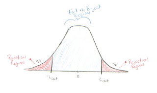
Acceptance Region - Opposite of the Rejection Region. It is better to call this the "Fail to Reject Region." In the case of a two-tailed hypothesis t-test, it is shaded in light blue on the picture below. If the test statistic falls between -tcritical and tcritical then we fail to reject the null hypothesis.

Adjusted R-Squared, R-Squared Adjusted - A version of R-Squared that has been adjusted for the number of predictors in the model. R-Squared tends to over estimate the strength of the association especially if the model has more than one independent variable.

Alpha [A, a ], Chosen Significance Level - The maximum amount of chance a statistician is willing to take that they will do not accept a null hypothesis that is true (Type I Error).

Alpha Error, Type I Error - An error made by wrongly rejecting the null hypothesis when the null is really true.

Alternative Hypothesis, Research Hypothesis - An hypothesis that does not conform to the one being tested, usually the opposite of the null hypothesis. Symbolized.

Analysis of Variance (ANOVA) - A test of differences between mean scores of two or more groups with one or more variables.

Approximation Curve, Curve Fitting - the general method for using a line or curve to estimate the relationship between two associated numerical variables.

Autocorrelation - This occurs when later variables in a time series are correlated with earlier variables.

B

Backward Elimination - A method of determining regression equation that starts with a regression equation that includes all independent variables and then remover variables that are not useful one at a time

Best Subsets Regression - A method of determining the regression equation used with statistical computer applications that allows the user to run multiple regression models using a specified number of independent variables. The computer will sort through all of the models and display the "best" subsets of all the models that were run. "Best" is typically identified by the highest value of R-squared. Other diagnostic statistics such as R-square adjusted and Cp are also displayed to help the user determine their best choice of a model.

Bell-Shaped Curve - A symmetrical curve. Looks like the cross-section of a bell.

Best Fit, Goodness of Fit - A model that is the best model for the given data.

Beta Error, Acceptance Error, Type II Error - An error made by wrongly accepting the null hypothesis when the null is really false.

Bivariate Association/ Relationship - The relationship between two variables only.

C

Cp Statistic - Cp measures the differences of a fitted regression model from a true model, along with the random error. When a regression model with p independent variables contains only random differences from a true model, the average value of Cp is (p+1), the number of parameters. Thus, in evaluating many alternative regression models, our goal is to find models whose Cp is close to or below (p+1).

Cook’s Distance: Cook’s distance combines leverages and studentized residuals into one overall measure of how unusual the predictor values and response are for each observation. Large values signify unusual observations. Geometrically, Cook’s distance is a measure of the distance between coefficients calculated with and without the ith observation. Cook and Weisberg suggest checking observations with Cook’s distance > F (.50, p, n-p), where F is a value from an F-distribution.

Coefficient of Determination – In general the coefficient of determination measures the amount of variation of the response variable that is explained by the predictor variable(s). The coefficient of simple determination is denoted by r-squared and the coefficient of multiple determination is denoted by R-squared.

Coefficient of Variation – The coefficient of variation, in regression, is the standard deviation of the predictor variable divided by the mean of the predictor variable. If this value is small, your variation in the y-values (predictor values) is nearly constant. This implies that the data are ill-conditioned.

Confidence Bands (Upper & Lower) - This is the range of the responses that can be expected for all of the appropriate inputs of X's. The upper confidence band is the highest value that the ÿh value is predicted to be. The lower confidence band is the lowest value predicted that ÿh could be.

Confidence Level - This is the amount of error allowed for the model (given as a percent or a).

Confidence Intervals - A range of values to estimate a value of a population parameter. Associated with the range of values is also the amount of confidence the researcher has in the estimate. For example, we might estimate the cost of a new space vehicle to be 35 million dollars. Assume that the confidence level is 95% and the margin of error is 5 million dollars. We say that we are 95% confident that the cost is between 30 and 40 million dollars.

Confidence Interval Bounds, Upper and Lower - The lower endpoint on a confidence interval is called the lower bound or lower limit. The lower bound is the point estimate minus the margin of error. The upper bound is the point estimate plus the margin of error.

Correlation - The amount of association between two or more items. In these tutorials, correlation will refer to the amount of association between two or more numerical variables.

Correlation Coefficients, Pearson’s Sample Correlation Coefficient, r - Measures the strength of linear association between two numerical variables.

Correlation Matrix - A table that shows all pairs of correlations coefficients for a set of variables.

Correlation Ratio- A kind of correlation used when the relation between two variables is assumed to be curvilinear (i.e. not linear).

Curve Fitting, Approximation Curve - the general method for using a line or curve to estimate the relationship between two associated numerical variables.

D

Degrees of Freedom, df, - The number of values that can vary independently of one another. For example, if you have a sample of size n that is used to evaluate one parameter, then there are n-1 degrees of freedom.

Dependent Variable, Response Variable, Output Variable - The variable in correlation or regression that cannot be controlled or manipulated. The variable that "depends" on the values of one or more variables. In math, y frequently represents the dependent variable.

DFITS, DFFITS: Combines leverage and studentized residual (deleted t residuals) into one overall measure of how unusual an observation is. DFITS is the difference between the fitted values calculated with and without the ith observation, and scaled by stdev (Ŷi). Belseley, Kuh, and Welsch suggest that observations with DFITS >2Ö(p/n) should be considered as unusual

Dummy Variable, Indicator Variable - A variable used to code the categories of a measurement. Usually, 1 indicates the presence of an attribute and 0 indicates the absence of an attribute. Example: If the measurement variable is cost of space flight vehicle then the vehicle might be manned or unmanned. Let the dummy variable be 1 if the vehicle is manned and 2 if it is unmanned. Note: Dummy variable coding can be used for more than 2 categories.

E

Efficiency, Efficient Estimator - It is a measure of the variance of an estimate's sampling distribution; the smaller the variance, the better the estimator.

Error - In general, the error difference in the observed and estimated value of a parameter.

Errors, Residuals - In regression analysis, the error is the difference in the observed Y values and the predicted Y values that occur from using the regression model. See the graph below.

Error, Specification (Specification error) - A mistake made when specifying which model to use in the regression analysis. A common specification error involves including a irrelevant variable and leaving out an important variable.

F

F (F test statistic) - This is the test statistic for whenever conducting an analysis of variance.

Fits, Fitted Values, Predicted Values - The Fits are the predicted values found by substituting the original values for the independent variable(s) into the regression equation. The name "fit" refers to how well the observed data matches the relationship specified in the model.

Forward Selection - A frequently available option of statistical software applications. A method of determining the regression equation by adding variables to the regression equation until the addition of new variables does not appear to be worthwhile.

F-test: An F-test is usually a ratio of two numbers, where each number estimates a variance. An F-test is used in the test of equality of two populations. An F-test is also used in analysis of variance, where it tests the hypothesis of equality of means for two or more groups. For instance, in an ANOVA test, the F statistic is usually a ratio of the Mean Square for the effect of interest and Mean Square Error. The F-statistic is very large when MS for the factor is much larger than the MS for error. In such cases, reject the null hypothesis that group means are equal. The p-value helps to determine statistical significance of the F-statistic.

G

General Linear Model (GLM) - A full range of methods used to study linear relations between one continuous dependent variable and one or more independent variables, whether continuous or categorical. “General” means the kind of variable is not specified. Examples include Regression and ANOVA.

H

Heteroscedasticity - Non constant error variance. Hetero = different; scedasticity = tendency to scatter.

Hierarchical Regression Analysis - A multiple regression analysis method in which the researcher, not a computer program, determines the order that the variables are entered into and removed from the regression equation. Perhaps the researcher has experience that leads him/her to believe certain variables should be included in the model and in what order.

Homoscedasticity - Constant error variance. Homo = same; scedasticity = tendency to scatter.

Hypothesis Testing - This is the common approach to determining the statistical significance of findings.

I

Independent Variable, Explanatory Variable, Predictor Variable, Input Variable - The variable in correlation or regression that can be controlled or manipulated. In math, x frequently represents the independent variable.

Influential Observation - An observation that has a large effect on the regression equation. Note: Outliers and leverage points may be influential observations, but influential observations are usually outliers and leverage points.

Intercorrelation - Correlation between variables that are all independent (no dependent variables involved).

L

Least Squares Regression - Regression analysis method which minimizes the sum of the square of the error as the criterion to fit the data. This can refer to linear or curvilinear regression.

Leverages, Leverage Points - An extreme value in the independent (explanatory) variable(s). Compared with an outlier, which is an extreme value in the dependent (response) variable.

Linear Correlation- A relationship between the independent and dependent data, that whenever plotted forms a straight line.

Linear Regression - Typically when regression is used without qualification, the type of regression is assumed to be linear regression. This is the method of finding a linear model for the dependent variable based on the independent variable(s).

M

Mean Square Residual, Mean Square Error (MSE) - A measure of variability of the data around the regression line or surface.

Measurement Error (Error, Measurement) - inaccurate results due to flaw(s) in the measuring instrument.

Multicollinearity, Collinearity - The case when two or more independent variables are highly correlated. The occurrence of multicollinearity can cause difficulties in multiple regression. If the independent variables are interrelated, then it may be difficult or impossible to find the specific effect of only one independent variable.

Multiple Correlation Coefficient, R - A measure of the amount of correlation between more than two variables. As in multiple regression, one variable is the dependent variable and the others are independent variables. The positive square root of R-squared.

Multiple Correlation - Correlation with one dependent variable and two or more independent variables. Measures the combined influences of the independent variables on the dependent. gives the proportion of the variance in the dependent variable that can be explained by the action of all the independent variables taken together.

Multiple Correlation Matrices - A table of correlation coefficients that shows all pairs of correlations of all the parameters with in the sample.

Multiple Correlation Plots - A collection of scatterplots showing the relationship between the variables of interest.

Multiple R - That is the name MS Excel uses for the Multiple Correlation Coefficient, R.

Multiple Regression, Multiple Linear Regression - A method of regression analysis that uses more than one independent (explanatory) variable(s) to predict a single dependent (response) variable. Note: The coefficients for any particular explanatory variable is an estimate of the effect that variable has on the response variable while holding constant the effects of the other predictor variables. “Multiple” means two or more independent variables. Unless specified otherwise, “Multiple Regression” generally refers to “Linear” Multiple Regression.

Multiple Regression Analysis (MRA) - Statistical methods for evaluation the effects of more than one independent variable on one dependent variable.

N

Negative Correlation- This occurs whenever the independent variable increases and the dependent variable decreases. This is also called a negative relationship.

Nonadditivity - A statement used to describe a relation when the addition of the separate effects do not add up to the total effect.

Nonlinearity - The events are not the same as their causes.

Nonlinear Relationship - A relationship between two variables for which the points in the corresponding scatterplot do not fall in approximately a straight line. Nonlinearity may occur because there is not a defined relationship between the variables as in the first figure below, or because there is a specific curvilinear relationship. See the parabolic relationship shown in the second graph below.

Normality Plot, Normal Probability Plot - A graphical representation of a data set used to determine if the sample represents an approximately normal population. A graph from Minitab is shown below. The sample data is on the x-axis and the probability of the occurrence of that value assuming a normal distribution is on the y-axis. If the resulting graph is approximately a straight line, then the distribution is approximately normal. There are statistical hypothesis tests for normality as well.

Null Hypothesis, - This is the hypothesis that two or more variables are not related and the researcher wants to reject.

O

Outlier - An extreme value in the dependent (response) variable. Compared with a leverage point, which is an extreme value in the independent (explanatory) variables.

P

Partial Correlation - Correlation between two variables given that the linear effect of one or more other variables has been controlled. Example. r12.3 is the correlation of variables one and two given that variable three has been controlled.

Partial Correlation Coefficients - This is the square root of a coefficient of partial determination. It is given the same sign as that of the corresponding regression coefficient in the fitted regression function.

Partial Determination Coefficients- This measures the marginal contribution of one X variable when all others are already included in the model. In contrast, the coefficient of multiple determination, , measures the proportion reduction in the variation of Y achieved by the introduction of the entire set of X variables considered in the model.

Partial Regression Coefficient, Partials - In a multiple regression equation, the coefficients of the independent variables are called partial regression coefficients because each coefficient tells only how the dependent variable varies with the selected independent variable.

Pearson’s Sample Correlation Coefficient, r - Measures the strength of linear association between two numerical variables.

Population - A group of people that one whishes to describe or generalize about.

Predictor Variable, Independent Variable, Explanatory Variable, Input Variable - The variable in correlation or regression that can be controlled or manipulated. In math, x frequently represents the independent variable.

Prediction Equation - An equation that predicts the value of one variable on the basis of knowing the value of one or more variables. Note: Formally prediction equation is a regression equation that does not include an error term.

Prediction Interval - In regression analysis, a range of values that estimate the value of the dependent variable for given values of one or more independent variables. Comparing prediction intervals with confidence intervals: prediction intervals estimate a random value, while confidence intervals estimate population parameters.

Population Parameter, Parameter - A measurement used to quantify a characteristic of the population. Even when the word population is not used with parameter, the term refers to the population. Example: The population mean is a measure of central tendency of the population. The population parametric is usually unknown.

Proportional Reduction of Error (PRE) - A measure of association that calculates how much more you can reduce your error in the predication of y if you know x, then when you do not know x. Pearson’s r is not a PRE, but r-squared is a PRE.

Positive Correlation- This relationship occurs whenever the dependent variable increases as the independent variable increases

P-values, Observed Significance Level - The probability of making a Type I error. (i.e. given that the null is true, the probability of getting a data set like the one we have or one more extreme in the direction of the alternative.)

R

r, Correlation Coefficients, Pearson’s r - Measures the strength of linear association between two numerical variables.

R, Coefficient of Multiple Correlation - A measure of the amount of correlation between more than two variables. As in multiple regression, one variable is the dependent variable and the others are independent variables. The positive square root of R-squared.

r2 , r-squared (r-sq.), Coefficient of Simple Determination - The percent of the variance in the dependent variable that can be explained by of the independent variable.

R-squared, Coefficient of Multiple Determination - The percent of the variance in the dependent variable that can be explained by all of the independent variables taken together.

R-Squared Adjusted (R-sq. adj.), Adjusted R-Squared - A version of R-Squared that has been adjusted for the number of predictors in the model. R-Squared tends to over estimate the strength of the association especially if the model has more than one independent variable.

Range of Predictability, Region of Predictability - The range of independent variable(s) for which the regression model is considered to be a good predictor of the dependent variable. For example, if you want to predict the cost of a new space vehicle subsystem based on the weight, and all of the input data subsystem weights all range from 100 to 200 pounds. You could not expect the resulting model to provide good predictions for a subsystem that weighs 3000 pounds.

Regression Analysis, Statistical Regression, Regression - Methods of establishing an equation to explain or predict the variability of a dependent variable using information about one or more independent variables. The equation is often represented by a regression line, which is the straight line that comes closest to approximating a distribution of points in a scatter plot. When "regression" is used without any qualification it refers to “linear” regression.

Regression Artifact, Regression Effect - An artificial result due to statistical regression or regression toward the mean.

Regression Coefficient, Regression Weight - In a regression equation the number in front of an independent variable. For example, if the regression equation is Y = mx + b then m is the regression coefficient of the x-variable. The regression coefficient estimates the effect of the independent variable(s) on the dependent variable. (Compare with Partial Regression Coefficients)

Regression Constant - Unless specified otherwise, the regression constant is the intercept in the regression equation.

Regression Equation - An algebraic equation that models the relationship between two (or more) variables. If the equation is Y = a + bX + e, then Y is the dependent variable, X is the independent variable, b is the coefficient of X, and a is the intercept, and e is the error term (See Prediction Equation).

Regression Line, Trend Line - When the best fitting regression model is a straight line, that line is called a regression “line.” Ordinary Least Squares method is usually used for computing the regression line.

Regression Model - An equation used to describe the relationship between a continuous dependent variable, an independent variable or variables, and an error term.

Regression Plane - When the regression model has two independent variables, then a plane represents the relationship between the variables two-dimensional. Example: z = a + bx + cy

Regression SS (also SSR or SSregression) - The sum of squares that is explained by the regression equation. Analogous to between-groups sum of squares in analysis of variance.

Regression Toward the Mean - The type of bias described by Francis Galton, a 19th century researcher. A tendency for those who score high on any measure to get somewhat lower scores on a subsequent measure of the same thing- or, conversely, for someone who has scored very low on some measure to get a somewhat higher score the next time the same thing is measured. Knowing how much regression toward the mean there is for a particular pair of variables gives you a prediction. If there is very little regression, you can predict quite well. If there is a great deal of regression, you can predict poorly if at all.
Regression Weight, Regression Coefficient - In a regression equation the number in front of an independent variable. For example, if the regression equation is Y = mx + b then m is the regression coefficient of the x-variable. The regression coefficient estimates the effect of the independent variable(s) on the dependent variable. (Compare with Partial Regression Coefficients)

Regress On - The dependent variable is “regressed on” the independent variable(s). We will regress the cost of the space vehicle (based) on the weight of the vehicle. If x predicts y, then y is regressed on x. (i.e. Regress the dependent variable on the independent. Response variable is regressed on the explanatory variable.)

Rejection Region - The area in the tail(s) of the sampling distribution for a test statistic. The figure below shows the Rejection Region in red.

Residuals, Errors - The amount of variation on the dependent variable not explained by the independent variable.

Response Variable- Same as the independent variable.

Robust - Said of a statistic that remains useful even when one or more of the assumptions is violated.

S

Sample - A group of subjects selected from a larger group, the population.

Sample Statistic, Statistic - A measurement used to quantify a characteristic of the Sample. Even when the word sample is not used, the term statistic refers to the sample. Example: The sample mean is a measure of central tendency of the sample (see Population Parametric).

Sampling Error, Sampling Variability, Random Error - The estimation of the expected differences between the sample statistic and the population parameter.

Sampling Distribution - It is all possible values of a statistic and their probabilities of occurring for a sample of a particular size.

Scaling - expresses the centered observation in the units of the standard deviation of the observations.

Scatter Diagram, Scattergram, Scatter Plot - The pattern of points due to plotting two variables on a graph.

Significance - The degree to which a researcher’s finding is meaningful or important.
Significance Level - there are two types of significance levels, the observed significance level (alpha) and the chosen significance level (p-value). The lower the probability the greater the statistical significance, called alpha level.

Simple Linear Regression - A form of regression analysis, which has only one independent variable.

Slope - The rate at which the line or curve rises or falls when covering a given horizontal distance.

Spearman Correlation Coefficient (rho), Rank-Difference Correlation, rs. - A statistical measure of the amount of monotonic relationship between two variables that are arranged in rank order.

Specification error (Error, Specification) - A mistake made when specifying which model to use in the regression analysis. A common specification error involves including a irrelevant variable and leaving out an important variable.

Standard Deviation - A statistic that shows the square root of the squared distance that the data points are from the mean.

Standardized Measure of Scale - Any statistic that allows comparisons between things measured on different scales. Example: percent, standard deviations and z-scores

Standardized Regression Coefficient - Regression Coefficients which have been standardized in order to better make comparisons between the regression coefficients. This is particularly helpful when different independent variables have different units.
Standardized Regression Model - This is the regression model used after centering and scaling of the dependent variable and independent variables.

Standardized residuals - Standardized residuals are of the form (residual) / (square root of the Mean Square Error). Standardized residuals have variance 1. If the standardized residual is larger than 2, then it is usually considered large.

Standard Error, Standard Error of the Regression, Standard Error of the Mean, Standard Error of the Estimate - In regression the standard error of the estimate is the standard deviation of the observed y-values about the predicted y-values. In general, the standard error is a measure of sampling error. Standard error refers to error in estimates resulting from random fluctuations in samples. The standard error is the standard deviation of the sampling distribution of a statistic. Typically the smaller the standard error, the better the sample statistic estimates of the population parameter. As N goes up, so does standard error.

Statistical Significance - Statistical significance does not necessarily mean that the result is clinically or practically important. For example, a clinical trial might result is a statistically significant finding (at the 5% level) that shows the difference in the average cholesterol rating for people taking drug A is lower than that of those taking drug B. However, drug A may only lower the cholesterol by 2 units more than drug B which is probably not a difference that is clinically important to the people taking the drug. Note: Large sample sizes can lead to results that are statistically significant that would otherwise be considered inconsequential.

Stepwise Regression - A method of regression analysis where independent variables are added and removed in order to find the best model. Stepwise regression combines the methods of backward elimination and forward selection.

Strength of Association, Strength of Effect Index - The degree of relationship between two (or more) variables. One example is R-squared, which measures the proportion of variability in a dependent variable explained by the independent variable(s).

Studentized Residuals: The studentized residual has the form of error/standard deviation of the error. Studentized residuals have constant variance when the model is appropraite.

T

Transformations - This is a method of changing all the values of a variable by using some mathematical operation.

U

Unbiased Estimator - A sample statistic that is free from systemic bias.

V

Variance Inflation Factor (VIF) - A statistics used to measuring the possible collinearity of the explanatory variables.

W

Weighted Least Squares - A method of regression used to take into account the non constant variance. The variables are multiples by a particular number (weights). It is typical to choose weights that are the inverse of the pure error variance in the response. (Minitab, page 2-7.) This choice gives large variances relatively small weights and visa versa.

Y

Y-intercept - is the point where a regressin line intersects the y axis.

Read more

Probability Applied to Landing Page Testing

So how does probability apply to landing page optimization?

The random variables are the visits to your site from the traffic sources that you have selected for the test. The audience itself may be subject to sampling bias. You are counting whether or not the conversion happened as a result of the visit. You are assuming that there is some underlying and fixed probability of the conversion happening, and that the only other possible outcome is that the conversion does not happen (that is, a visit is a Bernoulli random variable that can result in conversion, or not).

As an example, let's assume that the actual conversion rate for a landing page is 2%. Hence there is a larger chance that it will not convert (98%) for any particular visitor. As you can see, the sum of the two possible outcome probabilities exactly equals 1 (2% + 98% = 100%) as required.

The stochastic process is the flow of visitors from the traffic sources used for the test. Key assumptions about the process are that the behavior of the visitors does not change over time, and that the population from which visitors are drawn remains the same. Unfortunately, both of these are routinely violated to a greater or lesser extent in the real world. The behavior of visitors changes due to seasonal factors, or with changing sophistication and knowledge levels about your products or industry. The population itself changes based on your current marketing mix. Most businesses are constantly adjusting and tweaking their traffic sources (e.g., by changing PPC bid prices and the resulting keyword mix that their audience arrives from). The result is that your time series, which is supposed to return a steady stream of yes or no answers (based on a fixed probability of a conversion), actually has a changing probability of conversion. In mathematical terms, your time series is nonstationary and changes its behavior over time.

The independence of the random variables in the stochastic process is also a critical theoretical requirement. However, the behavior on each visit is not necessarily independent. A person may come back to your landing page a number of times, and their current behavior would obviously be influenced by their previous visits. You might also have a bug or an overload condition where the actions of some users influence the actions that other users can take. For this reason it is best to use a fresh stream of visitors (with a minimal percentage of repeat visitors if possible) for your landing page test audience. Repeat visitors are by definition biased because they have voluntarily chosen to return to your site, and are not seeing it for the first time at random. This is also a reason to avoid using landing page testing with an audience consisting of your in-house e-mail list. The people on the list are biased because they have self-selected to receive ongoing messages from you, and because they have already been exposed to previous communications.

The event itself can also be more complicated than the simple did-the-visitor-convert determination. In an e-commerce catalog, it is important to know not only whether a sale happened, but also its value. If you were to tune only for higher conversion rate, you could achieve that by pushing low-margin and low-cost products that people are more likely to buy. But this would not necessarily result in the highest profits.

Statistical Methods

Landing page testing is a form of experimental study. The environment that you are changing is the design of your landing page. The outcome that you are measuring is typically the conversion rate. Landing page testing and tuning is usually done in parallel, and not sequentially. This means that you should split your available traffic and randomly alternate the version of your landing page shown to each new visitor. A portion of your test traffic should always see the original version of the page. This will eliminate many of the problems with sequential testing.

Observational studies, by contrast, do not involve any manipulation or changes to the environment in question. You simply gather the data and then analyze it for any interesting correlations between your independent and dependent variables.

For example, you may be running PPC marketing programs on two different search engines. You collect data for a month on the total number of clicks from each campaign and the resulting number of conversions. You can then see if the conversion rate between the two traffic sources is truly different or possibly due to chance.

Descriptive statistics only summarize or describe the data that you have observed. They do not tell you anything about the meaning or implications of your observations. Proper hypothesis testing must be done to see if differences in your data are likely to be due to random chance or are truly significant.

Have I Found Something Better?

Landing page optimization is based on statistics, and statistics is based in turn on probability theory. And probability theory is concerned with the study of random events. But a lot of people might object that the behavior of your landing page visitors is not "random." Your visitors are not as simple as the roll of a die. They visit your landing page for a reason, and act (or fail to act) based on their own internal motivations.

So what does probability mean in this context? Let's conduct a little thought experiment.

I have flipped the coin and covered up the result after catching it in my hand. Now imagine if I peeked at the coin without letting you see it. What would you estimate the probability of it coming up heads to be? Still 50%, right? How about me? I would no longer agree with you. Having seen the outcome of the flip event I would declare that the probability of coming up heads is either zero or 100% (depending on what I have seen).

How can we experience the same event and come to two different conclusions? Who is correct? The answer is—both of us. We are basing our answers on different available information. Let's look at this in the context of the simplest type of landing page optimization. Let's assume that you have a constant flow of visitors to your landing page from a steady and unchanging traffic source. You decide to test two versions of your page design, and split your traffic evenly and randomly between them.

In statistical terminology, you have two stochastic processes (experiences with your landing pages), with their own random variables (visitors drawn from the same population), and their own measurable binary events (either visitors convert or they do not). The true probability of conversion for each page is not known, but must be between zero and one. This true probability of conversion is what we call the conversion rate and we assume that it is fixed.

From the law of large numbers you know as you sample a very large number of visitors, the measured conversion rate will approach the true probability of conversion. From the Central Limit Theorem you also know that the chances of the actual value falling within three standard deviations of your observed mean are very high (99.7%), and that the width of the normal distribution will continue to narrow (depending only on the amount of data that you have collected). Basically, measured conversion rates will wander within ever narrower ranges as they get closer and closer to their true respective conversion rates. By seeing the amount of overlap between the two bell curves representing the normal distributions of the conversion rate, you can determine the likelihood of one version of the page being better than the other.

One of the most common questions in inferential statistics is to see if two samples are really different or if they could have been drawn from the same underlying population as a result of random chance alone. You can compare the average performance between two groups by using a t-test computation. In landing page testing, this kind of analysis would allow you to compare the difference in conversion rate between two versions of your site design. Let's suppose that your new version had a higher conversion rate than the original. The t-test would tell you if this difference was likely due to random chance or if the two were actually different.

There is a whole family of related t-test formulas based on the circumstances. The appropriate one for head-to-head landing page optimization tests is the unpaired one-tailed equal-variance t-test. The test produces a single number as its output. The higher this number is, the higher the statistical certainty that the two outcomes being measured are truly different.

Collecting Insufficient Data

Early in an experiment when you have only collected a relatively small amount of data, the measured conversion rates may fluctuate wildly. If the first visitor for one of the page designs happens to convert, for instance, your measured conversion rate is 100%. It is tempting to draw conclusions during this early period, but doing so commonly leads to error. Just as you would not conclude a coin could never come up tails after seeing it come up heads just three times, you should not pick a page design before collecting enough data.

The laws of probability only guarantee the accuracy and stability of results for very large sample sizes. For smaller sample sizes, a lot of slop and uncertainty remain.

The way to deal with this is to decide on your desired confidence level ahead of time. How sure do you want to be in your answer—90%, 95%, 99%, even higher? This completely depends on your business goals and the consequences of being wrong. If a lot of money is involved, you should probably insist on higher confidence levels.

Let's consider the simplest example. You are trying to decide whether version A or B is best. You have split your traffic equally to test both options and have gotten 90 conversions on A, and 100 conversions on B. Is B really better than A? Many people would answer yes since 100 is obviously higher than 90. But the statistical reality is not so clear-cut.

Confidence in your answer can be expressed by means of a Z-score, which is easy to calculate in cases like this. The Z-score tells you how many standard deviations away from the observed mean your data is. Z=1 means that you are 67% sure of your answer, Z=2 means 95.28% sure, and Z=3 means 99.74% sure.

Pick an appropriate confidence level, and then wait to collect enough data to reach it.

Let's pick a 95% confidence level for our earlier example. This means that you want to be right 19 out of 20 times. So you will need to collect enough data to get a Z-score of 2 or more.

The calculation of the Z-score depends on the standard deviation ([.sigma]). For conversion rates that are less than 30%, this formula is fairly accurate:

In our example for B, the standard deviation would be 10

So we are 67% sure (Z=1) that the real value of B is between 90 and 110 (100 plus or minus 10). In other words, there is a one out of three chance that A is actually bigger than the lower end of the estimated range, and we may just be seeing a lucky streak for B.

Similarly at our current data amounts we are 95% sure (Z=2) that the real value of B is between 80 and 120 (100 plus or minus 20). So there is a good chance that the 90 conversions on A are actually better than the bottom end estimate of 80 for B.

Confidence levels are often illustrated with a graph. The error bars on the quantity being measured represent the range of possible values (the confidence interval) that would be including results within the selected confidence level. Figure 1: shows 95% confidence error bars (represented by the dashed lines) for our example. As you can see, the bottom of B's error bars is higher than the top of A's error bars. This implies that A might actually be higher than B, despite B's current streak of good luck in the current sample.

 Figure 1: Confidence error bars (little data)

If we wanted to be 95% sure that B is better than A, we would need to collect much more data. In our example, this level of confidence would be reached when A had 1,350 conversions and B had 1,500 conversions. Note that even though the ratio between A and B remains the same, the standard deviations have gotten much smaller, thus raising the Z-score. As you can see from Figure 2, the confidence error bars have now "uncrossed," so you can be 95% confident that B actually is better than A.

Figure 2: Confidence error bars (more data)

Read more